An advanced time series forecasting application implementing real ARIMA (AutoRegressive Integrated Moving Average) models with mathematical precision. This client project features their custom frontend design enhanced with a fully functional backend system for accurate sales predictions and statistical analysis.
This Sales Forecasting System is a client-commissioned project where they provided the initial frontend design and requirements. My role was to transform their vision into a fully functional application by implementing the complete backend architecture and mathematical algorithms.
The system implements genuine ARIMA methodology with real mathematical formulas including Yule-Walker equations for AR parameter estimation, Levinson-Durbin algorithm for efficient Toeplitz matrix solving, and Method of Moments for MA parameter estimation. Unlike simplified forecasting tools, this application performs actual statistical computations to deliver professional-grade time series analysis.
Built with Python Flask for robust backend processing and a modern JavaScript frontend using Chart.js for interactive visualizations. The system processes CSV time series data, applies differencing transformations, estimates model parameters through maximum likelihood methods, generates multi-step forecasts with confidence intervals, and provides comprehensive residual diagnostics including ACF/PACF analysis and Ljung-Box statistics.
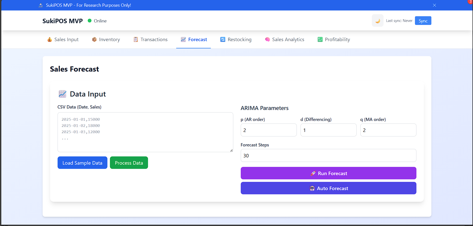
Genuine ARIMA(p,d,q) modeling with mathematical algorithms: Yule-Walker equations, Levinson-Durbin algorithm, and Method of Moments.
AR parameters via Yule-Walker/Levinson-Durbin, MA parameters through moment matching with Newton-Raphson refinement.
Automatic application of d-order differencing to achieve stationarity in time series data before modeling.
Generate forecasts for 1 to 100+ steps ahead with proper error propagation and confidence interval calculations.
Calculate forecast standard errors and confidence bounds using theoretical ARIMA variance formulas.
Complete residual analysis with mean, variance, standard deviation, and visual scatter plots for model validation.
Autocorrelation Function (ACF) visualization with up to 20 lags for model adequacy assessment.
Statistical test for autocorrelation in residuals using Q-statistic: Q = n(n+2) ╬Ż[Žü┬▓(k)/(n-k)].
AIC (Akaike Information Criterion) and BIC (Bayesian Information Criterion) for comparing different ARIMA specifications.
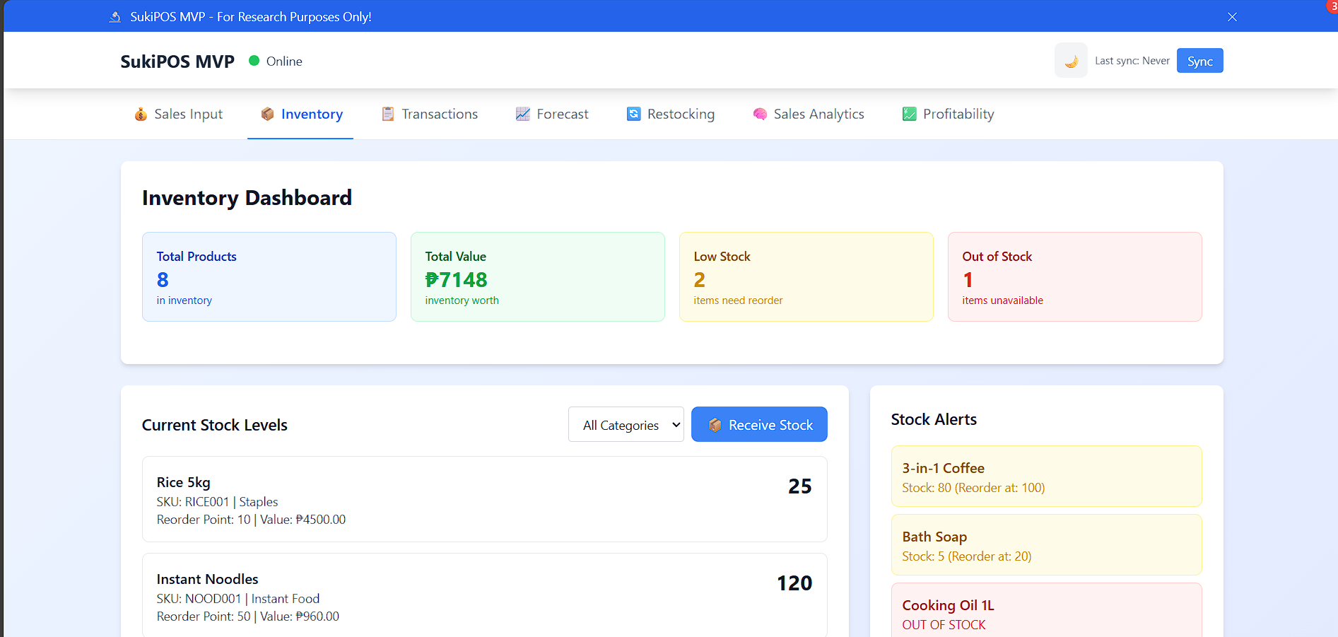
Import time series data from CSV files with date parsing and validation. Supports 10 to 1000+ data points.
Built-in generator creating realistic time series with trend, seasonality, AR components, and Gaussian noise.
Dynamic Chart.js graphs showing historical data, forecasts, confidence intervals, residuals, and ACF plots.
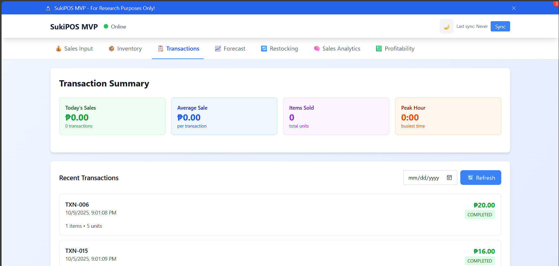
Tabular display of each forecast point with date, predicted value, standard error, and confidence bounds.
Adjust ARIMA(p,d,q) parameters manually with real-time formula display showing the current model equation.
Live rendering of ARIMA equation: Ōłć^d X_t = ŽåŌéüX_{t-1} + ... + ŽåŌéÜX_{t-p} + ╬Ą_t + ╬ĖŌéü╬Ą_{t-1} + ... + ╬ĖŌéæ╬Ą_{t-q}
Calculate model log-likelihood: Ōäō = -n/2┬Ęlog(2ŽĆ) - n/2┬Ęlog(Žā┬▓) - 1/(2Žā┬▓)┬Ę╬Ż╬Ą┬▓
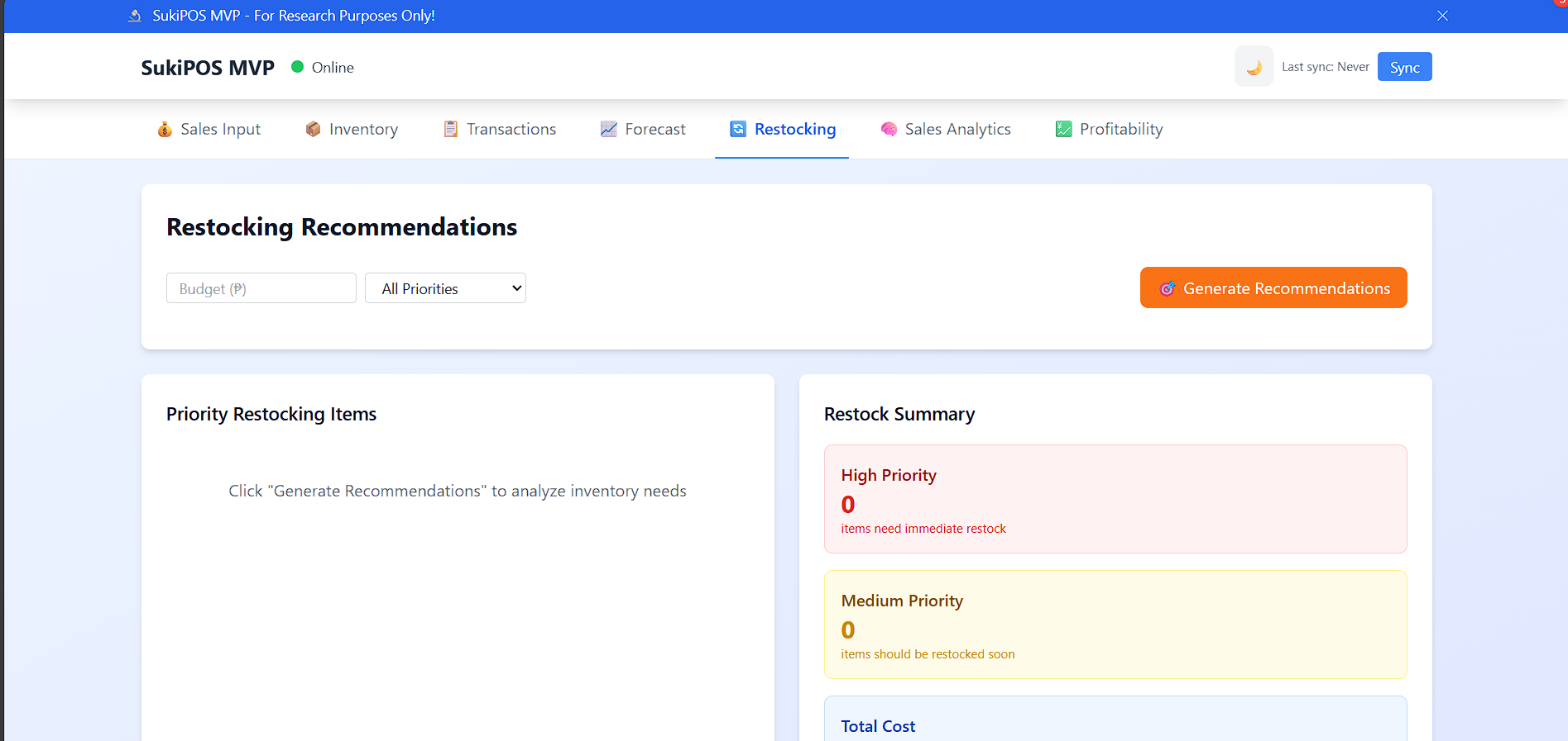
Properly handles non-stationary data through differencing, preserving long-term trends and seasonal patterns.
Client's custom frontend design optimized for desktop and mobile viewing with smooth animations.
Real-time feedback during data processing, parameter estimation, and forecasting with success/error messages.
Object-oriented JavaScript implementation with proper separation of concerns and modular Flask backend.